Before we start

This is a short tutorial to discuss the basic Markdown syntax and essential features of R Markdown to an R user with no experience in Markdown.

`R` refers to both the programming language and the free software environment for data analysis and graphics. RStudio is a popular environment (IDE, or integrated development environment) to only write your R scripts but also to interact with the R software. R Markdown is a file format for making dynamic, report-quality documents with R.

This blog post requires preliminary knowledge of using R in RStudio. If you want to quickly pick them up, this article about Introduction to R & RStudio can help with that.

What is Markdown?

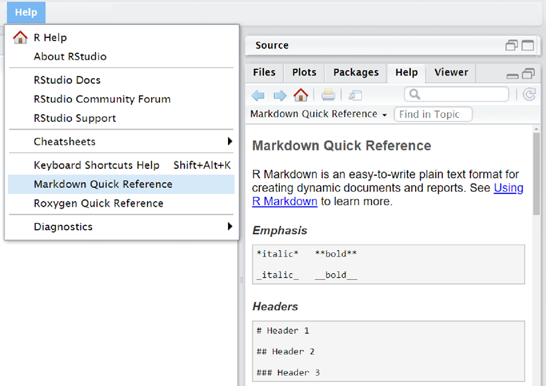
Markdown is a simple formatting syntax for authoring HTML, PDF, and MS Word documents. It is easy to format headings, bold text, italics, etc. There is quick reference for Markdown in RStudio as shown in Figure 1.

I summarized some mostly used syntax for Markdown here:

1. Emphasis: * or **
2. Headers: #, ##, and ###
3. Lists:
   1. Unordered list: -, +, etc…
   1. Ordered list: 1, 2, etc…
4. Links: [My personal website](https://yuxiaoluo.github.io)
5. Images: ![alt text](figures/img.png)
6. Horizontal Rule/Page Break: ******

Figure 2 shows the markdown syntax for the R User Group Introduction on GitHub and Figure 3 shows the rendered result of that.

What is R Markdown

R Markdown is a file format, which is written in Markdown (a plain text format) and contains chunks of R code. R Markdown provides an authoring framework for data science and can be used to save/execute code and generate high quality reports to share with audiences. R Markdown is popular because it is reproducible and supports dozens of static and dynamic output formats, such as pdf, html, latex, and so on.

Get started with R Markdown

First, we need to install the `rMarkdown` package to use it.

install.packages("rMarkdown")
library(rMarkdown)

Then, we can navigate to the Menu bar and open a new R Markdown file by clicking on these button in order File-> New File -> R Markdown…. An R Markdown file will be created and it comes with a suffix .Rmd.

R code chunks

One of the biggest benefits of R Markdown is that you can organize both the code and regular text in one document and code chunk is the place where you put the R code in. You can think of the code chunk as a single piece of R script and the code can do anything as it is in a R script file, such as reading data, data wrangling, constructing regression model, generating graphics, etc.

You can create an R code chunk by clicking the green button on top right as shown in Figure 4. Ctrl+Alt+i is the shortcut for creating R code chunk. You can also create code chunks executing other programming languages like Python, Bash, SQL, etc.

Embedding R code

You can embed an R code chunk and type R code in the chunk. It’s important to remember when you create an R Markdown file and if you run code to refer to an object, you should include instructions showing what is that object.

A = c("a", "a", "b", "b")
B = c(5, 9, 85, 23)
dataframe = data.frame(A, B)
print(dataframe)

If you are loading a data frame from a .csv file, you must include the code in .Rmd, like what you do in the normal R script.

dataframe = read.csv("~/Desktop/Code/dataframe.csv")

Including plots

When you want to include a plot without showing the R code that generates the plot. You can change the parameter to echo = FALSE.

```{r pressure, echo = FALSE}
plot(pressure)
```

Chunk options

R Markdown is using knitr to generate the .md file. There are more than 50 chunk options that can be used to fine-tune the behavior of knitr when processing R chunks. Please refer to the online documentation here for the full list of options.

You can apply the chunk options to individual code chunks; You can also apply any chunk options globally to a whole document, so you don’t have to repeat the options in every single code chunk. To set chunk options globally, call knitr::opts_chunk$set() in a code chunk (usually the first one in the document), like the first code chunk in this R Markdown document.

knitr::opts_chunk$set(
  comment = "#", echo = FALSE, fig.width = 6
)

Here I also listed 4 most useful code chunk options:

• eval: (TRUE; logical or numeric) Whether to evaluate the code chunk. It can also be a numeric vector to choose which R expression(s) to evaluate, e.g., eval = c(1, 3, 4) will evaluate the first, third, and fourth expressions, and eval = -(4:5) will evaluate all expressions except the fourth and fifth.
• echo: (TRUE; logical or numeric) Whether to display the source code in the output document. Besides `TRUE/FALSE`, which shows/hides the source code, we can also use a numeric vector to choose which R expression(s) to echo in a chunk, e.g., echo = 2:3 means to echo only the 2nd and 3rd expressions, and echo = -4 means to exclude the 4th expression.
• warning: (TRUE; logical) Whether to preserve warnings (produced by warning()) in the output. If FALSE, all warnings will be printed in the console instead of the output document. It can also take numeric values as indices to select a subset of warnings to include in the output. Note that these values reference the indices of the warnings themselves (e.g., 3 means “the third warning thrown from this chunk”) and not the indices of which expressions are allowed to emit warnings.
• include: (TRUE; logical) Whether to include the chunk output in the output document. If FALSE, nothing will be written into the output document, but the code is still evaluated and plot files are generated if there are any plots in the chunk, so you can manually insert figures later.

Output R Markdown file

Now you want to generate the markdown file. There are two ways to output your R Markdown file and render it to a new file in the format that we are familiar with, like webpage, pdf, etc. The first way of output is to click the Knit button in RStudio IDE, then a document will be generated that includes both content as well as the output of any embedded R code chunks within the document. R Markdown generates a new file that contains selected text, code, and results from the .Rmd file. The new file can be a web page, PDF, MS Word document, slide show, notebook, handout, book, dashboard, package vignette or other format.

The second way is to write the render() function in the RStudio console, where you can set output_format argument to render your .Rmd file to any R Markdown’s supported format. The code below renders 1-example.Rmd to a MS Word document.

library(rmarkdown)
render("1-example.Rmd", output_format = "word_document")

In the render process, R Markdown feeds the .Rmd file to knitr, which executes all of the code chunks and creates a new Markdown (.md) document which includes the code and its output. R Markdown can be rendered to different formats and to more than one type of documents at the same time by specifying one or more formats in the output argument.

If you do not select a format, R Markdown renders the file to its default format, which you can set in the output field of a .Rmd file’s header. The header of a raw R Markdown script shows that it renders to an HTML file by default. This article summarizes seven most useful formats in the list below, but it doesn’t include all the possible formats, you can find more other possible formats here.

• html_notebook – Interactive R Notebooks
• html_document – HTML document w/ Bootstrap CSS
• pdf_document – PDF document (via LaTeX template)
• word_document – Microsoft Word document (docx)
• odt_document – OpenDocument Text document
• rtf_document – Rich Text Format document
• md_document – Markdown document (various flavor)

RUG (R User Group)

If you have any questions regarding R or just want to simply get started with it, do not hesitate to join us at the RUG (R User Group) meetings or to schedule a consultation with the GC Digital Fellows.

Reference

The content of this blog post is inspired and adapted from the following public materials, many thanks to these authorsVisit these resources if you want to learn more about R Markdown.

R for Health Data Science by Ewen Harrison and Riinu Pius

R Markdown Lesson from RStudio

Getting started with R Markdown by John

R Markdown: The Definite Guide by Yihui Xie, J. J. Allaire, and Garrett Grolemund