As a form of data visualization, mapping is an informative way to explore and communicate our data and results. However, transforming information into a map-ready dataset is not always an intuitive task. Even when we have coordinates, or locality names, associated with what we collected or summarized, it may be daunting to understand how digital tools transform rows and columns into boundaries, shapes and colors. In this post, I will go through some basic questions to keep in mind when organizing your data in a map-friendly format.

1. Which geometry (or geometries) do you want to use?

In order to transform your spreadsheet into a map, the first question you need to answer is: which geometry do you want to use? In less formal terms, the question is: how do you want to show the information? Is the information better shown as points? As lines? Different boundaries? A gradient of colors changing through space? Answering this question will help you realize what format of spatial data you need to use, and from there understand how you should format your original data to be mapped using that geometry. One good thing is: usually the final structure of the data you will end up with will be universally usable across different digital tools, so your data will be ready to go regardless of the software you want to use, like QGIS, Tableau, ArcGIS, etc.

As a small example, I can bring some of the data I am working with right now in my PhD dissertation. I am currently extracting DNA from bird muscle tissues, and many of those tissues come to me from different natural history museums both within and outside the US. Therefore, the different spreadsheets they sent me with the data on the samples (what species it is, where it was collected, longitude and latitude) are far from standardized. One thing I like to do is visualize where those birds were originally collected, so I can decide whether I have enough samples for each species, or if I need to ask for more. The best way to represent this information is with a point geometry: each sampled locality can be represented as a point in my map. Luckily, the point geometry is the easiest one to format our data into. Thinking of a spreadsheet, I just need one row per sample, and at least two columns with longitude and latitude information (Fig. 1). When my spreadsheet is converted into a spatial file, each row becomes a feature of my point geometry file.

I may also want to include in my map how many samples I have per locality. Since more than one sample can have the same coordinate, I can make a spreadsheet where each row is a locality (i.e, the feature now is the locality, and not the sample), and then add a column where I will input the number of samples in each locality. These columns where I can add additional information about my feature is called an attribute. In fact, the spreadsheet you are making, with features as rows and attributes as columns, is called an attribute table (Fig. 2).

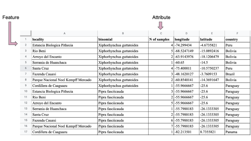
Notice how the dataset in figure 2 is similar to the one in figure 1, but they are organized in different ways: the basic unit to be mapped (i.e., the feature) is different in each case (sample in Figure 1, but Locality in Figure 2).

What if I wanted to have the amount of localities sampled, for instance, per state, instead of showing just the point localities? This would require me to change my geometry from point to polygon (since state boundaries are usually in polygons) and add the number of localities as a new attribute to that geometry. How to do that is what we are covering in the second question.

How to transform your data into a spatial file?

Most digital tools for mapping will require data in specific spatial formats. The two basic formats are vector data and raster data. You can learn more about them in this link, but for our conversation here, all you need to know is that vector files are a collection of spatial entities, the features, each associated to a different geometry that dictates how they will be plotted in space. The three basic kinds of geometries are points, lines and polygons. This understanding is important to figure out how we can create a vector file from our data.

Let’s use the quick example from above: if I have a spreadsheet with all my samples and their respective longitude and latitude, how can I make a map of states and color each state based on the number of localities in it? I would first need a vector file in polygon geometry that has the states information. I could create that file on my own or I could use an available file on the internet. Creating a polygon vector file on my own would require me to delineate the coordinates of all the vertices that together compose the polygons of the state I am interested in. That is doable, but it is a lot of work. Luckily, vector files with state information are very common on the internet, so we can just download one for the country we want, and figure out how to add our personal data information. One way to add this information is to perform what is called a Join operation; i.e., I have a polygon vector file, where each polygon is a different feature, and then I join to it a spreadsheet that has information on each of these polygons/features. I am essentially creating or expanding the attribute table of my polygon vector file. Here is a quick tutorial on how to do that by one of the former GC Digital Fellows.

Notice that, even though we are starting to combine different geometries with our data, everything starts and is dictated by our initial spreadsheet (our initial “attribute table”). This highlights the importance of starting and maintaining a well-organized dataset from the beginning, which is the topic of the next question.

What if I do not know what I want to map yet? Is there a way to universally organize my data so it is always organized and ready to go?

Since the answers to questions 1 and 2 may change for different questions or for different moments throughout your research, it is important to have your data organized in an intuitive way from the beginning. Intuitive in this context means intuitive more to your computer than to you. The best way to approach this organization task is to think of the most basic unit of information you will want to map: that would be your feature. When organizing your data, visualize each row as a separate observation about the phenomenon you study (be it animals in nature or students in a classroom). Think of each column as an additional type of information you can have about that specific observation. I personally like to make my data spreadsheets as conceptually broad as possible: I have a general focus for that spreadsheet, and I try to add as many columns as types of information that might be relevant for my research (specially in the beginning, when I am still in the process of thinking about my research questions).

Here is one example again from my own research. I work with some species of birds: I am interested in differences among these birds (e.g., size of the body, what they eat, where they live) as well as differences in their environment (e.g., type of climate, type of forest they live in, size of a forest fragment, etc.) and how those differences impact the size of a population. In the most raw sense, the information I am interested in is population size: that is my response variable and what I want to explain. So, in my data spreadsheet, each row could be a measured population size that I observed in nature. Then I can add, for that row, many columns, each giving important information about that observation: to which species it belonged, the method that was used to measure population size, if it is from a published study or my own data. Since I am also interested in differences among different species and different environments, I can also add those types of information: what the species eat, its size, where it lives, what kind of climate, etc.

Notice that this spreadsheet allows me to store my raw data and then derive any kind of information from it by using some data wrangling skills. For instance, if I have five populations (five rows) from the same species, I can easily get an average of population size for that species. I can also use, for instance, the climate column to split my data into species in warm weather vs species in cold weather, and then calculate average and test any differences statistically. The message here is that your spreadsheet can be as global as you want, and for further analyses you can just filter out the information you do not need.
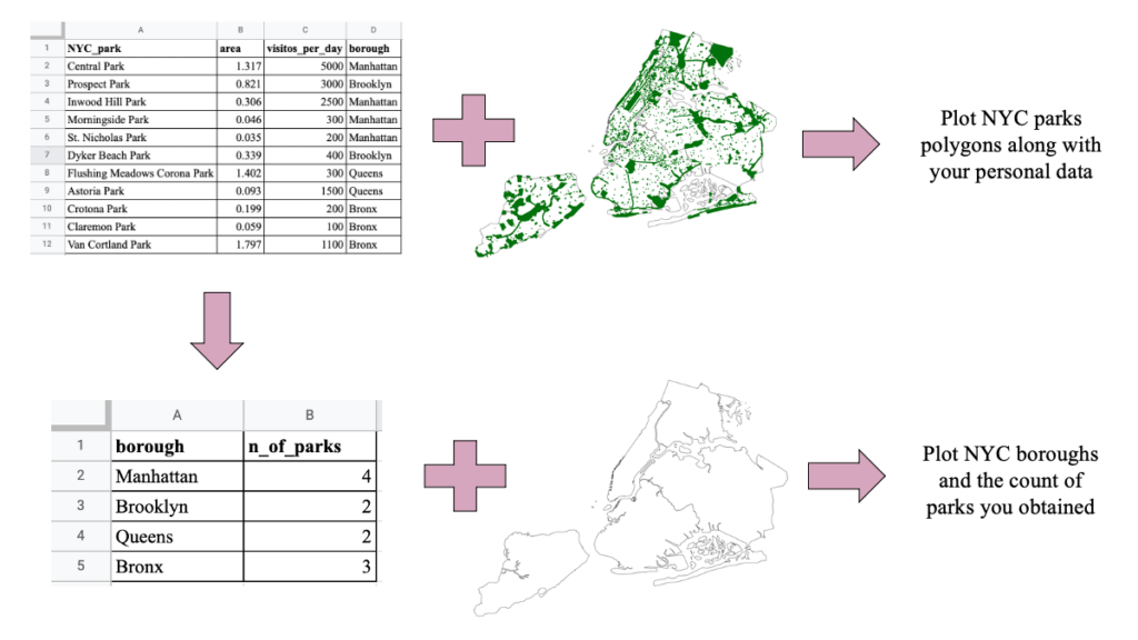
But since we are talking about mapping (or, better, data visualization), let’s see some examples of that. I can make my spreadsheet above be explicitly spatial by adding two columns for longitude and latitude. Now each population will have a spatial location associated with it. From that, my spreadsheet can be easily converted, for instance in GIS, to a spatial object with a point geometry. In other cases, like for instance if each row in my spreadsheet represents a different NYC park, maybe a polygon geometry would be the best. In this case, I can join my raw spreadsheet with a shapefile that already has the NYC parks polygons (as shown in question 2 above). Or maybe I want to know how many NYC parks exist per borough of the city: I can use the exact same original spreadsheet I have, if I have the column for boroughs somewhere. I can sum up how many times each borough repeats in my spreadsheet, that will give me the amount of parks per borough. That info can then be converted into a smaller spreadsheet (again, using some data wrangling skills) which can be joined to a shapefile that already has the borough polygons (Fig. 3). Notice how your original spreadsheet can be the starting point for many things, including, but not restricted to, maps.

Take home message is: organize your data in the most global, raw and uniform way possible. For that, think of how you can structure your data around the basic unit of information you are interested in (in maps, that would be your feature), and how additional info can be added about each unit as additional columns (in maps, that would be your attributes). This will allow you to derive your data to several applications in an easy way and save you a lot of time in the future.

This entry is licensed under a Creative Commons Attribution-NonCommercial-ShareAlike 4.0 International license.